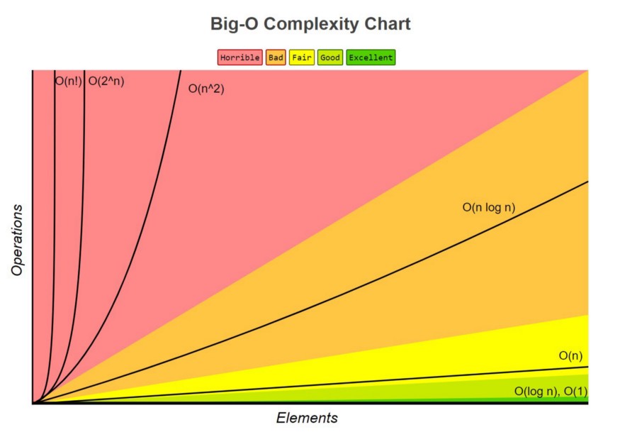
In the previous post, we have discussed the definitions of Computational Complexity, Big O Notation, and have been introduced to some common time complexities. We will discuss in details each of the common time complexities and example to understand more about how to calculate it.

1. Constant Time - O(1)

Algorithms that have constant time complexity are those do not depend on the size of the input data. The run time will remain the same not matter how big or small of the input data size.

For example, consider below example of an algorithm to get the first item:

constant pokemons = ['Bulbasaur', 'Squirtle', 'Charmander', 'Caterpie', 'Weedle'];
function getFirst(data) {
   console.log(data[0]);
}
 
getFirst(pokemons);

The function always have the same running time regardless of the input data size because it always get the first item of the list. An algorithms with constant time complexity is the best since we don't need to worry about the input size.

2. Logarithmic Time - O(log n)

Algorithms that have logarithmic time complexity are those do not need to iterate through every single element of the input data. In other word, an algorithm, which reduces the number of elements that it has to iterate through after each step, is considered to have logarithmic time complexity.

Binary search is a perfect example for logarithmic time complexity. If you don't know binary search, it's an algorithms to search for a number in a sorted list. Below are steps of the algorithm:

• Go to the middle element of the list first.
• If the searched value is lower than the value in the middle of the list, set a new right bounder.
• If the searched value is higher than the value in the middle of the list, set a new left bounder.
• If the search value is equal to the value in the middle of the list, return the middle (the index).
• Repeat the steps above until the value is found or the left bounder is equal or higher the right bounder.

Here is how it looks like in code:

const binarySearch = (array, target) => {
  let startIndex = 0;
  let endIndex = array.length - 1;
  while(startIndex <= endIndex) {
    let middleIndex = Math.floor((startIndex + endIndex) / 2);
    if(target === array[middleIndex) {
      return console.log("Target was found at index " + middleIndex);
    }
    if(target > array[middleIndex]) {
      console.log("Searching the right side of Array")
      startIndex = middleIndex + 1;
    }
    if(target < array[middleIndex]) {
      console.log("Searching the left side of array")
      endIndex = middleIndex - 1;
    }
    else {
      console.log("Not Found this loop iteration. Looping another iteration.")
    }
  }
   
  console.log("Target value not found in array");
}

If you are still confused, watch below video to understand the algorithm. 

Notice how the dancers are in a line with numbers on their backs. The man with the number seven on his back is looking for the woman who matches. He doesn’t know where she is but he knows all the ladies are in sorted order.

His process is to go to the dancer in the middle and ask her which side of her number seven is on. When she says: “She’s to the left of me,” he can rule out everyone to her right.

Next, he asks the woman in the middle of the left side the same question. This lets him rule out another half of the candidates and so on until he finds number seven.

As we can see, the binary search algorithm doesn't loop through each number of the input array. Instead, the iterated size reduced by half after each step of the algorithm. So, we can say this algorithm has logarithmic time complexity.

3. Linear Time - O(n)

An algorithm is said to have a linear time complexity when the running time increases at most linearly with the size of the input data. This is the best possible time complexity when the algorithm must examine all values in the input data. For example:

const data = [1,2,3,4,5,6];
function printAll(array) {
   for (let i = 0; i < array.length; i++) {
    console.log(array[i]);
  }
}
 
printAll(data);

Note that in this example, we need to look at all values in the list to print the value. So, we can say this function has linear time complexity.

4. Quasilinear Time - O(n log n)

An algorithm is said to have a quasilinear time complexity when each operation in the input data have a logarithmic time complexity. It is commonly seen in sorting algorithms.

Merge sort is a great example of an algorithm which has quasilinear time complexity. In merge sort, we perform by below steps to sort an array of number:

• Divide the unsorted list into N sub-lists, each containing 1 element.
• Take adjacent pairs of two singleton lists and merge them to form a list of 2 elements. N will now convert into N/2 lists of size 2.
• Repeat the process till a single sorted list of obtained.

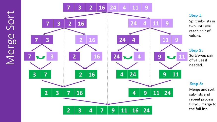
The list of size N takes maximum log N times to be halved into a singleton list, and the merging of all sublists into a single list takes N time, the worst case run time of this algorithm is O(N log N).

5. Quadratic Time - O(n²)

An algorithm is said to have a quadratic time complexity when it needs to perform a linear time operation for each value in the input data, for example:

const boxes = [1,2,3,4,5];
 
function logAllPairsOfArray(array){
   for(let i = 0; i < array.length; i++) {
      for(let j = 0; j < array.length; j++) {
         console.log(i, j);
      }
   }
}
 
logAllPairsOfArray(boxes);

If you see a nested loops like above, we use multiplication. So, the time complexity will be come O(n * n) or O(n²). We call this algorithm has quadratic time complexity. That means every time the number of elements increases, the operation time will increase quadratically. 

Bubble sort is a great example of quadratic time complexity since for each value it needs to compare to all other values in the list, let’s see an example:

let bubbleSort => (inputArr) {
    let len = inputArr.length;
    for (let i = 0; i < len; i++) {
        for (let j = 0; j < len; j++) {
            if (inputArr[j] > inputArr[j + 1]) {
                let tmp = inputArr[j];
                inputArr[j] = inputArr[j + 1];
                inputArr[j + 1] = tmp;
            }
        }
    }
    return inputArr;
};

6. Exponential Time - O(2ⁿ)

An algorithm is said to have an exponential time complexity when the growth doubles with each addition to the input data set. This kind of time complexity is usually seen in brute-force algorithms.

In cryptography, a brute-force attack may systematically check all possible elements of a password by iterating through subsets. Using an exponential algorithm to do this, it becomes incredibly resource-expensive to brute-force crack a long password versus a shorter one. This is one reason that a long password is considered more secure than a shorter one.

Another example of an exponential time algorithm is the recursive calculation of Fibonacci numbers:

function fibonacci(num) {
  if (num <= 1) return 1;
 
  return fibonacci(num - 1) + fibonacci(num - 2);
}

A recursive function may be described as a function that calls itself in specific conditions. As you may have noticed, the time complexity of recursive functions is a little harder to define since it depends on how many times the function is called and the time complexity of a single function call.

It makes more sense when we look at the recursion tree. The following recursion tree was generated by the Fibonacci algorithm using n = 4:

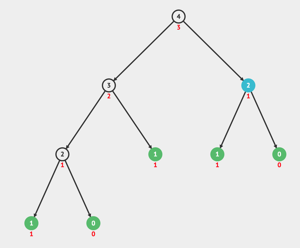
Note that it will call itself until it reaches the leaves. When reaching the leaves it returns the value itself.

Now, look how the recursion tree grows just increasing the n to 6:

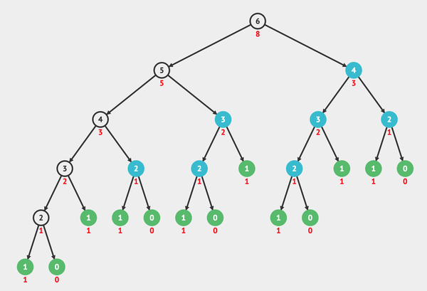
7. Factorial - O(n!)

An algorithm is said to have a factorial time complexity when it grows in a factorial way based on the size of the input data, for example:

2! = 2 x 1 = 2
3! = 3 x 2 x 1 = 6
4! = 4 x 3 x 2 x 1 = 24
5! = 5 x 4 x 3 x 2 x 1 = 120
6! = 6 x 5 x 4 x 3 x 2 x 1 = 720
7! = 7 x 6 x 5 x 4 x 3 x 2 x 1 = 5.040
8! = 8 x 7 x 6 x 5 x 4 x 3 x 2 x 1 = 40.320

let swap = function(array, index1, index2) {
  var temp = array[index1];
  array[index1] = array[index2];
  array[index2] = temp;
  return array;
};
 
let permutationHeap = function(array, result, n) {
  n = n || array.length; // set n default to array.length
  if (n === 1) {
    result(array);
  } else {
    for (var i = 1; i <= n; i++) {
      permutationHeap(array, result, n - 1);
      if (n % 2) {
        swap(array, 0, n - 1); // when length is odd so n % 2 is 1,  select the first number, then the second number, then the third number. . . to be swapped with the last number
      } else {
        swap(array, i - 1, n - 1); // when length is even so n % 2 is 0,  always select the first number with the last number
      }
    }
  }
};
 
//
var output = function(input) {
  console.log(input);
};
 
permutationHeap(["a", "b", "c"], output);

[1, 2, 3]
[2, 1, 3]
[3, 1, 2]
[1, 3, 2]
[2, 3, 1]
[3, 2, 1]